Processing PMRA Precipitation Data: From Satellite Rasters to Agricultural Insights

When evaluating fields for lease in Argentina, one question always comes up: how much rain does this area really get? The problem is that ground-based weather stations are sparse and don't cover most rural areas. Satellite data like ERA5 has low spatial resolution and questionable accuracy for local decisions.

The good news is that CONICET's PMRA (Precipitaciones Mensuales de la República Argentina) dataset solves this. It combines ground measurements with four global precipitation products using random forest regression. This gives us 5km resolution precipitation data for every corner of Argentina from 2000 to 2023.

But there's a challenge: the data comes as 288 individual raster files. One file per month for 24 years. Working with them one by one is impractical when you need to analyze trends, calculate statistics, or compare regions.

Why This Matters for Agricultural Operations

In my role leading innovation at an agricultural company, we constantly evaluate new land for lease. Understanding precipitation patterns is critical for:

Estimating crop yield potential in unfamiliar regions
Assessing drought risk for insurance decisions
Planning rotation strategies based on historical rainfall distribution

Without complete precipitation data, we're making expensive decisions with incomplete information. PMRA fills that gap, but only if we can process it efficiently.

The PMRA Dataset: What You're Working With

The PMRA dataset provides monthly precipitation data at 5km resolution across Argentina. Each GeoTIFF file covers the entire country for one month. The naming convention follows this pattern: PMRA_[month]_[year].tif.

Download the complete dataset from CONICET's Drive folder. You'll get 288 files totaling several gigabytes of precipitation data.

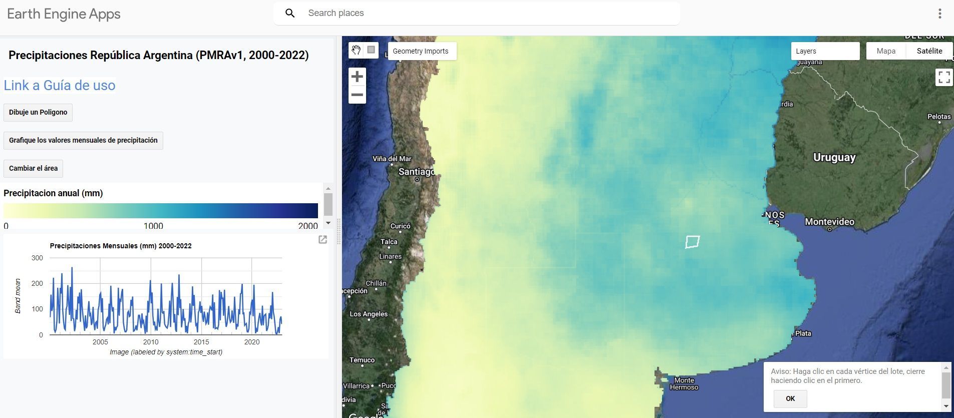
They also developed a Google Earth Engine app that lets you visualize the 23 annual precipitation maps, define an area of interest, and generate a chart of the monthly precipitation time series.

PMRA Precipitation Rasters

The key advantage over ERA5 or other satellite products is the combination of ground truth with satellite data. This hybrid approach delivers better local accuracy without requiring a weather station in your specific area.

Why XArray Changes Everything

Most GIS professionals are familiar with working with individual rasters using tools like rasterio or GDAL. The standard workflow looks like this:

Open raster file
Extract data
Process
Close file
Repeat 287 more times

This approach breaks down when you need to analyze temporal patterns. XArray treats your 288 rasters as a single multidimensional dataset organized by time, latitude, and longitude.

XArray Data Structure

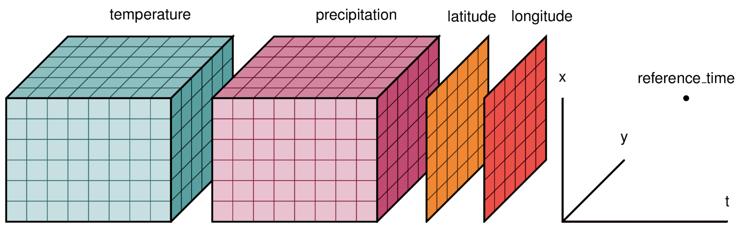
Instead of managing 288 file handles, you work with one unified data structure. This makes temporal queries instant: "What was the average precipitation in this location across all Januaries?" becomes a single line of code.

Setting Up the Environment

First, install the required libraries:

pip install rioxarray xarray numpy pandas geopandas matplotlib python-dotenv

The core imports for this workflow:

import rioxarray
import numpy as np
import xarray as xr
import matplotlib.pyplot as plt
import os, glob
from pathlib import Path
import pandas as pd
import geopandas as gpd
import rasterio
import datetime
from dotenv import load_dotenv

load_dotenv()
xr.set_options(keep_attrs=True, display_expand_data=False)

Loading and Organizing 288 Rasters

The first challenge is reading all raster files and organizing them chronologically. The file names contain the month and year, but we need to parse them into proper datetime objects.

rasters_path = os.getenv('RASTERS_PATH')

raster_files = str(Path(rasters_path) / '*.tif')
file_names = [os.path.basename(x) for x in glob.glob(raster_files)]
file_paths = [os.path.abspath(x) for x in glob.glob(raster_files)]

months_str_list = ['ene', 'feb', 'mar', 'abr', 'may', 'jun', 
                   'jul', 'ago', 'sep', 'oct', 'nov', 'dic']
months_num_list = range(1, 13)
my_dict = dict(zip(months_str_list, months_num_list))

dates = []
for file in file_names:
    file_name = Path(file).name
    month_str = file_name[5:8]
    year = file_name[-8:-4]
    for key, value in my_dict.items():
        if month_str == key:
            month = value
    date = pd.to_datetime(f'{year}-{month}')
    dates.append(date)

This extracts the Spanish month abbreviations and years from filenames, then converts them to Python datetime objects. These become the time dimension in our XArray dataset.

Building the XArray Dataset

Here's where XArray shows its power. Instead of looping through files, we concatenate all rasters along the time dimension in one operation:

time_var = xr.Variable('time', dates)

geotiffs_da = xr.concat([rioxarray.open_rasterio(i) for i in file_paths], 
                        dim=time_var)

geotiffs_ds = geotiffs_da.to_dataset("band")
geotiffs_ds = geotiffs_ds.rename({1: 'precipitacion'})

What we get is a Dataset with dimensions (time: 288, y: 851, x: 713). That's 288 months, 851 latitude points, and 713 longitude points. Every pixel now has a complete 24-year precipitation history.

The output structure looks like this:

<xarray.Dataset>
Dimensions:        (time: 288, y: 851, x: 713)
Coordinates:
  * x              (x) float64 -73.86 -73.82 -73.77 ... -52.75 -52.71 -52.66
  * y              (y) float64 -55.4 -55.36 -55.31 ... -21.22 -21.18 -21.13
    spatial_ref    int64 0
  * time           (time) datetime64[ns] 2001-05-01 2015-05-01 ... 2018-05-01
Data variables:
    precipitacion  (time, y, x) float32 nan nan nan nan nan ... nan nan nan nan

Exporting to NetCDF for Reusability

Once you've built the XArray dataset, save it as NetCDF. This is a self-describing binary format designed for scientific data:

out_file = Path(raster_files).parent.parent / 'precipitaciones_arg_PMRA.nc'
geotiffs_ds.to_netcdf(out_file)

NetCDF files preserve all metadata and load much faster than processing 288 individual rasters. The next time you need this data, you can load the entire 24-year dataset in seconds instead of minutes.

Converting to DataFrame for Analysis

XArray is great for spatial operations, but most analysis tools expect tabular data. Converting to a Pandas DataFrame gives you access to the full ecosystem of Python data science libraries:

precipitacion_df = geotiffs_ds.to_dataframe().reset_index()
precipitacion_df = precipitacion_df[['time', 'x', 'y', 'precipitacion']]
precipitacion_df = precipitacion_df.dropna()
precipitacion_df.precipitacion = precipitacion_df.precipitacion.astype('int8')

This creates a 40+ million row DataFrame with columns for time, coordinates, and precipitation values. Each row represents one pixel at one point in time.

The .dropna() step is important because many pixels fall outside Argentina's borders and contain null values. Removing them reduces file size and speeds up analysis.

Creating a GeoDataFrame for Spatial Analysis

If you need to perform spatial operations like overlays or spatial joins, convert to a GeoDataFrame:

from shapely.geometry import Point

precipitacion_df['geometry'] = [Point(xy) for xy in zip(precipitacion_df['x'], 
                                                         precipitacion_df['y'])]
gdf = gpd.GeoDataFrame(precipitacion_df)

This adds a geometry column with Point objects for each coordinate pair. Now you can:

Spatially join with field boundaries
Filter by region using polygons
Calculate zonal statistics for specific areas
Export to GIS formats like GeoPackage or Shapefile

out_file = Path(raster_files).parent.parent / 'precipitaciones_arg_PMRA.gpkg'
gdf.to_file(out_file, driver='GPKG')

Real-World Application: Field Evaluation

When we evaluate a potential lease field, I run this workflow to extract precipitation data for that specific location. The process takes minutes:

Load the field boundary as a polygon
Spatially filter the GeoDataFrame to points within the boundary
Group by time and calculate mean precipitation
Generate monthly and annual statistics
Compare against regional benchmarks

This gives us a 24-year precipitation history for a field we've never farmed. We can identify drought-prone years, calculate growing season rainfall, and assess variability.

Without PMRA data, we'd be relying on the nearest weather station, which might be 50km away in a different microclimate. With PMRA, we have site-specific data at 5km resolution.

Key Takeaways

You don't need weather stations to analyze precipitation anywhere in Argentina. PMRA provides validated, high-resolution data that combines the accuracy of ground measurements with the coverage of satellite data.

XArray is the right tool for this job because it handles multidimensional geospatial data natively. Trying to process 288 rasters individually is inefficient and error-prone.

The output formats matter. NetCDF for quick reloading, DataFrames for statistical analysis, GeoDataFrames for spatial operations. Choose the format that matches your downstream workflow.

Next Steps

If you're working with agricultural data in Argentina and need to incorporate precipitation analysis into your decision-making, this workflow is a starting point. The same approach works for other gridded time-series datasets like temperature, NDVI, or soil moisture.

I'm always interested in discussing how spatial data analysis can improve agricultural operations. If you're tackling similar challenges or want to explore how these techniques apply to your specific use case, let's connect.

Book Free Intro Call

You can also find me on LinkedIn where I share more about GIS, Python, and agricultural innovation.